2D Fundamentals¶
Overview¶
We treat the Purkinje network as a fractal tree. Each branch grows by adding short segments at its tip; the direction is steered by a repulsion field that keeps new points away from the already-built tree and preserves spacing. The page summarizes the growth rule used in the paper [1] and maps it to the library API.
Discrete growth rule¶
Let \(\mathbf{x}^i\) be the end point of the i-th segment of a branch and \(\mathbf{d}^i\) the unit direction of that segment. Growth proceeds by computing a new direction and then advancing a fixed step:
Where
\(d_{\mathrm{CP}}(\mathbf{x})\) is the distance to the closest point already in the tree, and \(\nabla d_{\mathrm{CP}}\) points in a repulsive direction.
\(w\) is the repulsion weight controlling how strongly tips avoid existing branches.
\(\ell_b\) is the branch length for the current generation.
\(N_s\) is the number of segments per branch; the step size is \(\ell_b/N_s\).
Initial direction at bifurcation. When a new branch is spawned, its first direction \(\mathbf{d}^1\) is obtained by rotating the parent’s last direction by the branching angle \(\pm \alpha_b\) within the local tangent plane. For subsequent segments, use ((1))–((2)).
Parameter mapping (paper → library)¶
\(\ell_b\) →
FractalTreeParameters.length(median branch length).\(\alpha_b\) →
FractalTreeParameters.branch_angle(branching angle).\(w\) →
FractalTreeParameters.w(repulsion weight).\(N_s\) → implicit via the step length:
FractalTreeParameters.l_segmentcontrols the step; typically \(N_s \approx \lceil \ell_b / \texttt{l\_segment} \rceil\).Segment spacing / collisions →
Nodes.collision(), with KD-tree updates viaNodes.update_collision_tree().
Implementation notes¶
The direction update is renormalized every step (unit vector).
Multiple branches may grow “in parallel” (one step at each active tip) until the current generation reaches \(N_s\) segments.
The geometric update is performed in a parameter space (2D chart) and projected back to the endocardial surface; see Projection to the Heart Surface.
Figure¶
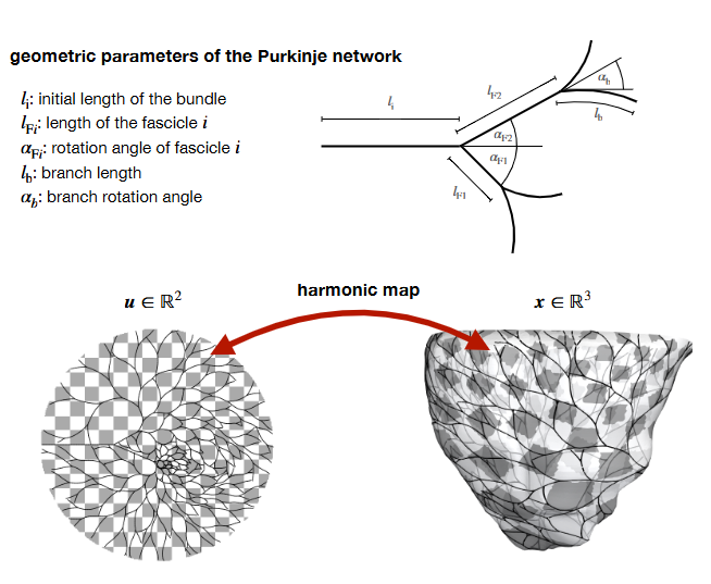
Fig. 3 Paper schematic of the growth process, showing the role of \(\ell_b\), \(\alpha_b\), and \(w\). See [1] §2.1.¶
API cross-reference¶
purkinje_uv.fractal_tree_uv.FractalTree– orchestrates growth (grow_tree), maintainsedges,connectivity,end_nodes.purkinje_uv.branch.Branch– computes the next step and requests projection/collision checks.purkinje_uv.mesh.Mesh–project_new_point,gradient,detect_boundary,compute_uvscaling(used during growth).purkinje_uv.nodes.Nodes– spacing control:collision,update_collision_tree.
Algorithm flow (generation loop)¶
        flowchart TD
  A([Start]) --> B[FractalTree.grow_tree()]
  B --> C[Init nodes/edges and seeds]
  C --> D{More generations?}
  D -->|Yes| E{Active tips left?}
  D -->|No| Z[Finalize: build PurkinjeTree(nodes, connectivity, end_nodes)]

  E -->|Pick tip t| F[Branch.step()]
  F --> G[Update direction d_next = normalize(d + w * grad dCP)]
  G --> H[Propose 2D step: l_b / N_s]
  H --> I[Map 2D to 3D candidate]
  I --> J[Mesh.project_new_point(candidate) -> x_proj]
  J --> K{Nodes.collision(x_proj)?}

  K -->|Too close| L{Reduce step?}
  L -->|Yes| H
  L -->|No| M[Terminate tip; mark end node]
  M --> E

  K -->|OK| N[Append node and Edge(n_prev, new)]
  N --> O{Reached N_s segments this generation?}
  O -->|No| E
  O -->|Yes| P{Bifurcate here?}
  P -->|Yes| Q[Spawn child tips with +/- branch_angle]
  Q --> E
  P -->|No| E

  Z --> END([Done])
Fig. 4 Algorithm flow for the fractal-tree generation loop.¶
Single step: class interaction¶
        sequenceDiagram
  participant FT as FractalTree
  participant BR as Branch
  participant ME as Mesh
  participant NO as Nodes

  FT->>BR: step()
  BR->>BR: compute d_next (w · grad d_CP)
  BR->>ME: project_new_point(candidate)
  ME-->>BR: x_proj
  BR->>NO: collision(x_proj)
  NO-->>BR: ok / too close
  alt ok
    BR-->>FT: append node & Edge(n_prev, new)
  else too close
    BR-->>FT: reduce step or terminate tip
  end
Fig. 5 One growth step — who calls whom.¶
References¶
[1] — Section 2.1 (Purkinje network generation), Figure 2.